Building a Neural Network with PyTorch

Building your first neural network could seem like a formidable undertaking, but deep learning frameworks like PyTorch have made the task more accessible than ever. In this article, I’ll explain how to build a neural network using PyTorch—even if you’re brand new to neural networks. We at Gcore recently developed a speech-to-text translation tool based on an advanced speech recognition ML model powered by our AI IPU cloud infrastructure, so I decided to focus the guide on building a neural network specifically for speech recognition.

Why Use PyTorch for Building Neural Networks?

Before delving into the how, let’s start with the why: Why specifically use PyTorch, rather than an alternative? Let’s be clear: There is no single “best” framework, “best” is subjective and context-dependent. Specific frameworks suit specific applications, such as FastAI for beginners or Keras for those who want a high-level API on top of TensorFlow. The TensorFlow framework itself shares many capabilities with PyTorch, but the straightforward and intuitive API from PyTorch renders it superior for prototyping and experimentation, like in this case.

Recent industry trends indicate a rising preference for PyTorch in research and production, attributed to its ease of debugging and intuitive tensor operations. On HuggingFace, 92% of models are exclusively PyTorch, up from 85% last year, compared to just 8% for TensorFlow. PyTorch’s CUDA compatibility further enhances its efficiency in handling large-scale speech datasets on GPUs. Evidently, PyTorch is an industry standard—and for good reason—rendering it a useful choice in a learning case such as this.

Building a Neural Network for Speech Recognition Using PyTorch

Let’s get to work and build a neural network for speech recognition using PyTorch. Within the steps, you’ll find sample code snippets for reference. Please note that speech recognition is a complex task. For real-world applications, more advanced models and techniques may be required.

Step 1: Environment Setup

First, install the PyTorch, TorchAudio, and NumPy libraries. There are other optional libraries you might need depending on the specific requirements of your project, like SciPy, SoundFile, Python Speech Features, Matplotlip, and Pandas. For instance, SoundFile is required for advanced audio file handling and you might need Pandas if you’re dealing with a lot of tabular data. For the core functionality to build a speech recognition model, TorchAudio and NumPy are sufficient.

Although you can install PyTorch using pip, we recommend choosing the appropriate version and installation steps based on your hardware (CPU & GPU) requirements, per PyTorch’s recommendation.

It’s better to create a virtual environment for your project using tools like venv or conda, instead of containerizing your environment or using a cloud-based one. A virtual environment allows you to keep your dependencies isolated from other projects and provides a clean environment so that you only install the dependencies you need for your project.

Here’s the code snippet to create a virtual environment and install required packages:

# Create a virtual environment (recommended)
python -m venv speech_recognition_env
source speech_recognition_env/bin/activate

# Install required packages
pip install torch torchaudio numpy matplotlib

Step 2: Data Collection

Obtain a dataset of audio files and transcriptions and organize it by using a consistent file naming convention and logical directory structures for files and folders, collecting and maintaining metadata, accurately mapping transcripts to their corresponding audio files.

To build your first neural network for speech recognition, I’d recommend using preprocessed datasets from open sources because it allows you to compare your results with existing benchmarks and helps to save time and effort in preprocessing vast amounts of data.

However, if you go for a raw or unprocessed dataset, include a variety of accents, ages, and recording conditions to make it diverse. Diverse datasets typically lead to better model accuracy since the model is more likely to have been trained on the relevant accent, auditory environment, etc.

Step 3: Data Preprocessing

Preprocess the audio data by using feature extraction, resampling, normalizing the audio/volume, and segmenting longer recordings into smaller, manageable parts.

Feature Extraction

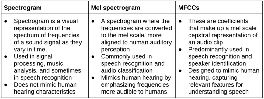
Feature extraction involves converting raw audio format into a format that ML models can understand. In this case, it means extracting features from the audio signal that are most relevant to recognizing speech. For feature extraction, you can convert the audio into spectrograms, mel spectrograms, or MFCCs (mel-frequency cepstral coefficients.) Here are the differences among these three methods of feature extraction:

While MFCCs are computationally less intensive than spectrograms and mel spectrograms, they may not capture some nuances of the speech signal. Spectrograms use high computational power and don’t emphasize the frequency bands most relevant to human speech. I recommend using mel spectrograms.

Segmenting Files

For segmenting audio files into smaller chunks, ensure that the length of segmented audio files is slightly shorter than the input limit of the model. The input limit varies across different language models and depends on the model architecture, the types of features and their dimensions extracted, available memory and processing power of the hardware, and the overall application of the speech recognition model. For example, our Whisper model has a limit of ~450 tokens, equivalent to about 30 seconds.

Downsampling Audio

It’s also a good idea to downsample the audio to a lower sampling rate for consistency across the dataset during model training. A lower sampling rate is required for speech recognition to ensure that the input to the model is uniform for efficient training; 16kHz is sufficient to capture details in human speech and it’s also computationally efficient. It can even capture frequencies below 8kHz accurately.

Here’s a sample code snippet for loading and preprocessing audio files:

import torchaudio
import os

# Example: Load and preprocess an audio file
filename = "path/to/audio.wav"
waveform, sample_rate = torchaudio.load(filename)

Mapping

Next, create a mapping between phonemes or words and their corresponding numerical labels:

1. Identify the set of phonemes (set of sounds that make up a language) and words you want the model to recognize. For words, use a vocabulary list relevant to your application or service.
2. Assign a numerical label to each phoneme and word in your set. For example, if you have 50 phonemes, you’ll assign numeric values of 0 to 49 to each phoneme.
3. Create a lookup table or dictionary where each phoneme and word is mapped to its corresponding numeric value.

Here’s a sample code to map phonemes or words to numeric labels:

vocab = {
    'zero': 0,
    'one': 1,
    'two': 2,
    # Add more entries for your vocabulary
}

Tokenizing and Encoding

Tokenize and encode the transcriptions using sequence-to-sequence models. Tokenization and encoding convert raw text into a structured format, allowing language models to learn the mapping between audio data and its corresponding textual format. Here’s how:

1. Create and configure a Byte Pair Encoding (BPE) tokenizer using the ‘ByteLevelBPETokenizer’ class from the ‘tokenizers’ library.
2. Use the ‘enable_truncation and enable_padding’ methods to set the maximum sequence length and enable truncation and padding of sequences to the specified length.
3. Train the tokenizer on a list of transcriptions using the ‘train_from_iterator’ method.
4. Save the trained tokenizer.
5. Load the saved tokenizer and process a list of transcriptions using the ‘encode_batch method’, which tokenizes and encodes the transcriptions.

And here’s a sample code snippet for tokenization and encoding:

from tokenizers import ByteLevelBPETokenizer
from tokenizers.processors import BertProcessing

# Define the paths to save tokenizer model files
tokenizer_model_path = "path/to/tokenizer"
tokenizer_config_path = "path/to/tokenizer-config.json"

# Initialize the BPE tokenizer
tokenizer = ByteLevelBPETokenizer()

# Customize tokenizer settings
tokenizer.enable_truncation(max_length=128)
tokenizer.enable_padding(max_length=128)
# Train the tokenizer on a list of transcriptions
transcriptions = ["This is a sample transcription.", "Another example for tokenization."]
tokenizer.train_from_iterator(transcriptions)

# Save the tokenizer model and configuration
tokenizer.save_model(tokenizer_model_path)
tokenizer.save(tokenizer_config_path)

# Load the saved tokenizer
tokenizer = ByteLevelBPETokenizer(tokenizer_model_path, tokenizer_config_path)

# Process transcriptions: Tokenize and encode
encoded_transcriptions = tokenizer.encode_batch(transcriptions)

# Display the tokenized and encoded results
for i, encoding in enumerate(encoded_transcriptions):
    print(f"Transcription {i + 1}:")
    print("Tokens:", encoding.tokens)
    print("Input IDs:", encoding.ids)
    print("Attention Mask:", encoding.attention_mask)
    print()

Best Practices

The following data preprocessing best practices will further improve your outcomes:

• Process data in batches to speed up training.
• If available, use GPUs for faster computation.
• Split the dataset into training, validation, and test sets. A common split ratio is 80% training, 10% validation, and 10% test.

Step 4: Dataset and DataLoader Creation

Next, create custom dataset classes by subclassing, which allows you to customize the behavior of your dataset class to meet the specific requirements of your project. A dataset class is a Python class that represents your dataset and provides an interface for accessing individual data samples. The dataset class is required to load the data (e.g., reading audio files, reading text) and to apply any necessary preprocessing (e.g., feature extraction, tokenization.) DataLoader divides the data into batches and shuffles the data to introduce randomness. Here’s how:

1. Create a custom Dataset class in PyTorch by inheriting from (subclassing) ‘torch.utils.data.Dataset’.
2. Implement the ‘__len__’ method to return the size of the dataset and ‘__getitem__’ to fetch an audio sample and its corresponding label.
3. Once you have your ‘Dataset’, use ‘torch.utils.data.DataLoader’ to handle batching, shuffling, and preparing data for parallel processing.

Here’s a sample code covering these steps:

from torch.utils.data import Dataset, DataLoader

class SpeechRecognitionDataset(Dataset):
    def __init__(self, audio_paths, transcriptions, vocab):
        self.audio_paths = audio_paths
        self.transcriptions = transcriptions
        self.vocab = vocab

    def __len__(self):
        return len(self.audio_paths)

    def __getitem__(self, idx):
        waveform, _ = torchaudio.load(self.audio_paths[idx])
        transcription = self.transcriptions[idx]
        target = [self.vocab[token] for token in transcription.split()]  # Convert text to numerical labels
        return waveform, target

# Create DataLoader
batch_size = 32
dataset = SpeechRecognitionDataset(audio_paths, transcriptions, vocab)
dataloader = DataLoader(dataset, batch_size=batch_size, shuffle=True)

In addition, I recommend creating a custom dataset class to encapsulate data loading and preprocessing logic in one place, making your code more manageable, and taking care to select an appropriate batch size matching available memory and hardware.

Step 5: Model Definition

Now, it’s time to define your neural network model. You can choose from various architectures, such as RNNs (recurrent neural networks,) CNNs (convolutional neural networks,) or transformer-based models. In this example, we’ll use a simple RNN-based module using PyTorch, simply because it’s the easiest to understand and implement. Perform the following steps:

• Define a neural network model class by inheriting from ‘torch.nn.Module’.
• Implement the ‘__init__’ method to define layers such as convolutional layers, recurrent layers (like LSTM or GRU,) and linear layers.
• Implement the ‘forward’ method to specify the forward pass of the network using the defined layers.

Here’s how that looks in code:

import torch.nn as nn

class SpeechRecognitionModel(nn.Module):
    def __init__(self, input_dim, hidden_dim, output_dim):
        super(SpeechRecognitionModel, self).__init__()
        self.rnn = nn.RNN(input_dim, hidden_dim, num_layers=2, batch_first=True)
        self.fc = nn.Linear(hidden_dim, output_dim)

    def forward(self, x):
        output, _ = self.rnn(x)
        logits = self.fc(output)
        return logits

You might want to consider using more advanced models such as LSTM, GRU, or Convolutional Neural Networks (CNNs,) depending on the complexity of your task and dataset. Also, adjust your model’s depth and width based on the available computational resources.

Step 6: Model Training

This step involves defining a training loop, optimizer, and loss function.

Loss function: Also known as a cost function or objective function, loss function quantifies how far off the model’s predictions are from the original target values (the desired accuracy level,) thus guiding the model during training to predict or classify data accurately.

Optimizer: The optimizer algorithm changes the attributes of the neural network, such as weights and learning rate, determining how quickly and accurately the model can converge.

Training loop: This is where the model actually learns to understand and transcribe spoken language.

• Write a training loop that iterates over the DataLoader for your training dataset.
• In each iteration, pass the input data through the model to obtain predictions, compute the loss, and perform backpropagation by calling ‘loss.backward()’.
• Update the model parameters with ‘optimizer.step()’ and clear the gradients with ‘optimizer.zero_grad()’.

Here’s how that looks in code:

# Instantiate the model
model = SpeechRecognitionModel(input_dim, hidden_dim, output_dim)

# Loss and optimizer
criterion = nn.CrossEntropyLoss()
optimizer = torch.optim.Adam(model.parameters(), lr=0.001)

# Training loop
num_epochs = 10
for epoch in range(num_epochs):
    for batch_inputs, batch_targets in dataloader:
        optimizer.zero_grad()
        logits = model(batch_inputs)
        loss = criterion(logits.view(-1, output_dim), batch_targets.view(-1))
        loss.backward()
        optimizer.step()
    print(f"Epoch [{epoch + 1}/{num_epochs}] Loss: {loss.item()}")

Step 7: Model Evaluation

The next important step in the process is to evaluate your model to understand how well the model is likely to perform on unseen or new data and find out if it meets the intended goal of the application.

• After each epoch (one complete pass through the entire training dataset,) evaluate your model on the validation set to monitor performance improvements.
• Use the Word Error Rate (WER) metric to assess the quality of your model’s transcriptions.
• Analyze types and patterns of errors for insights into what the model is learning and where it is failing.

It’s important to conduct multiple rounds of training and evaluation to assess the robustness and stability of the model.

The code for model evaluation could look like this:

import jiwer

# Validation loop
model.eval()
with torch.no_grad():
    total_wer = 0
    for batch_inputs, batch_targets in validation_dataloader:
        logits = model(batch_inputs)
        predicted_labels = logits.argmax(dim=-1)

        # Convert numerical labels back to text
        predicted_text = [list(vocab.keys())[list(vocab.values()).index(label)] for label in predicted_labels]
        predicted_text = " ".join(predicted_text)
        true_text = " ".join([list(vocab.keys())[list(vocab.values()).index(label)] for label in batch_targets])

        # Calculate WER
        wer = jiwer.wer(true_text, predicted_text)
        total_wer += wer

average_wer = total_wer / len(validation_dataloader)
print(f"Average WER: {average_wer}")

Step 8: Inference

When the model is trained, the final step is to use the trained model to predict the transcription of new, unseen audio data. Inference tests the model in a real-world scenario.

• Based on the model evaluation, select the model iteration that performed best to finalize the model.
• Apply the same preprocessing to the new data as implemented in previous steps and input the preprocessed data into the model.
• Convert the mode’s output into a human-readable format and use the output for further analysis and decision-making.
• Continuously monitor the model’s performance.
• Further update or retrain the model to maintain its accuracy over time.

Based on your requirements, you might need to further post-process the output (human-readable format) to correct mistakes like punctuation or formatting. The final output is the transcribed text from the audio input.

Your inference code could look like this:

# Load and preprocess a new audio sample
new_waveform, _ = torchaudio.load("path/to/new_audio.wav")

# Pass through the model
model.eval()

with torch.no_grad():
    logits = model(new_waveform.unsqueeze(0))  # Add batch dimension
    predicted_labels = logits.argmax(dim=-1)
    predicted_text = " ".join([list(vocab.keys())[list(vocab.values()).index(label)] for label in predicted_labels[0]])
    print(f"Predicted Text: {predicted_text}")

Conclusion

This guide should give you a good starting point to initiate your own projects based on PyTorch. However, keep in mind that this guide outlines only the basic framework for creating a speech recognition neural network using PyTorch—I highly recommend exploring advanced techniques and architectures, and learning to optimize the model for better accuracy and efficiency. For in-depth knowledge and skill development in PyTorch, you can explore the PyTorch resources.

The field of AI and machine learning is characterized by ongoing innovation and broader areas of application, including in natural language processing. Be sure to stay up to date with the latest research, best practices, and tools to leverage the full potential of deep learning frameworks!